At Drivy we have massively been using Redshift as our data warehouse since mid-2015, we store in it all our transformations and aggregations of our production database and 3rd-party data (spreadsheets, csv, APIs and so on). In this first blog post, we will discuss how we adapted our Redshift configuration and architecture as our usages changed over time.
This article targets a technical audience designing or maintaining Redshift data warehouses: architects, database developers or data engineers. It will aim to provide a simple overview, with a mix of tips to help you scale your Redshift cluster.
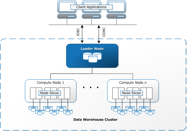
To recap, Amazon Redshift is a fully managed, petabyte-scale data warehouse deployed on AWS. It is based on PostgreSQL 8.0.2, uses columnar storage and massively parallel processing. It also has a very good query plan optimizer and strong compression capabilities.

In this first blog post, we will cover the following topics:
The big picture is that we have different usages with different SLA levels: from fast-running queries that must be highly available (near real-time reporting for fraud) to long-running batch jobs (e.g: propagating an ID on all the tracking records for all the sessions of all the users across all their devices 😅).
Prior to recent changes, Redshift was subject to roughly 50K requests per day:
Since a few months ago our usages have slightly changed as more analysts came and a new set of exploratory tools is being used.
We’ve decided to deploy Tableau to all project managers and analysts to improve agility in data-driven decision making. They have started using it with their own credentials to ingest data from Redshift to Tableau.
It resulted in multiplying the concurrent connections to Redshift by two, and a high load on the queue dedicated to analysts, neither fitting the current WLM strategy, therefore breaking our SLAs.
We identified a few levers.
Initially we had the following workload management strategy, in addition to the Short Query Acceleration queue set at a maximal timeout of 6 seconds:
| queue | concurrency | timeout | RAM |
|---|---|---|---|
| etl | 5 | ∞ | 50% |
| visualisations | 5 | 900s | 20% |
| analysts | 3 | 900s | 20% |
| default | 2 | 1800s | 10% |
When enabled, Redshift uses machine learning to predict short running queries and affect them to this queue, so there is no need to define and manage a queue dedicated to short running queries, for more info.
To face the limitations introduced by the use of Tableau through the credentials of the analysts, we’ve created a dedicated Redshift user group called exploration where we’ve added the Tableau user, using the same Redshift queue as the etl and slightly changed the timeout of the other ones to the following configuration:
| queue | concurrency | timeout | RAM |
|---|---|---|---|
| etl, exploration | 5 | ∞ | 50% |
| visualisations | 4 | 1500s | 20% |
| analysts | 4 | 1800s | 20% |
| default | 2 | 3600s | 10% |
We kept the SQA queue and increased its timeout to 20s. This avoids short queries getting stuck behind the long-running ones in the visualisations, analysts and default queues.
This new configuration limited the high load on the analysts queue resulting in queries being queued and frequent out of memory issues, but added some lag on the ETL pipelines.
We wanted to monitor badly designed queries, and queries that are subject to a bad distribution of the underlying data, significantly impacting the queries execution time. WLM gives us the possibility to define rules for logging, re-routing or aborting queries when specific conditions were met.
We decided to log all the queries that may contain errors, such as badly designed joins requiring a nested loop (cartesian product between two tables).
Here is an example of our current logging strategy:

When the rules are met, the query ID is logged in the STL_WLM_RULE_ACTION internal table.
Here is a view to locating the culprit: the query text, the user or system who ran it and the rule name that it is violating (defined in the WLM json configuration file).
CREATE OR REPLACE VIEW admin.v_wlm_rules_violations AS
SELECT
    distinct usename,
    "rule",
    "database",
    querytxt,
    max(recordtime) as last_record_time
FROM STL_WLM_RULE_ACTION w
INNER JOIN STL_QUERY q
ON q.query = w.query
INNER JOIN pg_user u
on u.usesysid = q.userid
group by 1, 2, 3, 4;
Note that the query rules are executed in a bottom-up approach, if 3 rules are defined (log, hop and abort).
The query will be logged and then re-routed to the next available queue (⚠️ only for SELECT and CREATE statements) before being aborted.
Now that we have a suitable workload configuration and a few monitoring tools to log badly designed queries, let’s see how to improve query performances to shorten the ETL pipelines!
The only way of approximating it is to define the correct combination of distribution and sort keys.
Here is a recipe for choosing the best sort keys, adapted from AWS documentation:
interleaved distribution style.And, for distribution keys:
The explain command gives us the opportunity to test different distribution styles by measuring the query cost.
To summarize, using explain it’s really important to follow certain points.
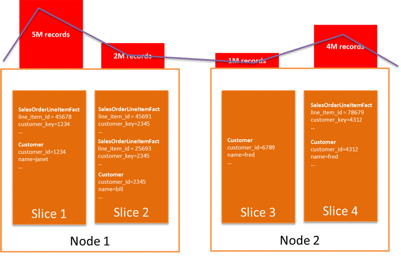
You should also be careful regarding the skew ratio across slices of your worker nodes if you have an interleaved sort distribution style, if the data is evenly distributed the load is split evenly across slices of each worker.

Bonus tip: this view gives you a full overview of all the tables in your database and it gives, the following information on each table:
CREATE OR REPLACE VIEW admin.v_tables_infos as
SELECT
  SCHEMA schemaname,
  "table" tablename,
  table_id tableid,
  size size_in_mb,
  CASE
    WHEN diststyle NOT IN ('EVEN','ALL') THEN 1
    ELSE 0
  END has_dist_key,
  CASE
    WHEN sortkey1 IS NOT NULL THEN 1
    ELSE 0
  END has_sort_key,
  CASE
    WHEN encoded = 'Y' THEN 1
    ELSE 0
  END has_col_encoding,
  CAST(max_blocks_per_slice - min_blocks_per_slice AS FLOAT) / GREATEST(NVL (min_blocks_per_slice,0)::int,1) ratio_skew_across_slices,
  CAST(100*dist_slice AS FLOAT) / (SELECT COUNT(DISTINCT slice) FROM stv_slices) pct_slices_populated
FROM svv_table_info ti
JOIN (
  SELECT
    tbl,
    MIN(c) min_blocks_per_slice,
    MAX(c) max_blocks_per_slice,
    COUNT(DISTINCT slice) dist_slice
    FROM (
      SELECT
        b.tbl,
        b.slice,
        COUNT(*) AS c
      FROM STV_BLOCKLIST b
      GROUP BY b.tbl, b.slice)
    WHERE tbl IN (SELECT table_id FROM svv_table_info)
    GROUP BY tbl) iq
ON iq.tbl = ti.table_id;This not-too-long blog post highlighted some of the straight forward ways to scale a Redshift cluster, by configuring the best WLM setup, leveraging query rules monitoring and improving query performances by limiting redistribution.
You should also bear the following list of various points in mind when designing your data warehouse:
SCAN operation will take more time;On the last major update of Redshift, Amazon came up with Redshift Spectrum. It is a dedicated Amazon Redshift server independent from the main cluster. Such as many compute intensive tasks can be pushed down to the Amazon Spectrum layer using Amazon S3 as its storage. It uses much less of the cluster’s processing and storage resources and provides unlimitedish read concurrency!
We will deep dive in Redshift Spectrum in the second part of this blog post series.
Meanwhile, don’t hesitate of course to reach me out for any feedback!